A few years ago, I obtained an OBDII scan tool/dynamometer simulation/calculation program that can graph volumetric efficiency (VE) over rpms.

Using real world vehicles, and no useful instructions, I devised a test sequence that allows a technician to see things another way.

What is Volumetric Efficiency?

Let’s keep this simple to start. An engine is an air pump and has a predictable volume of air that it can move.
The throttle plate has a high pressure side and a low pressure side. Air that is outside the throttle plate will have no effect on engine mechanical until it first passes though the intake manifold.

The MAF sensor is mounted in front of it all. Incoming air measured by the MAF is proportionate to the air flowing through the exhaust.
Unwanted exhaust restrictions lower VE and produces a back pressure in the exhaust. Intake flow restrictions will reduce VE without producing a back pressure.

VE is also a good diagnostic tool for finding air that might be entering the intake system after the MAF sensor.
How the Test Was Performed

To perform these tests the right way, a level road or parking lot is needed. First, with the throttle closed, coast between 10 to 20 mph. Next, go to wide open throttle for the entire test.

All of the vehicles in this article are gasoline port-injected, automatic transmissions unless otherwise stated. Vehicle setup conditions vary slightly from car to car. Some benefit from a subtle incline in the road as road grade and starting speed affect the rising edge.

The rising edge of the intake opening event will be nearly digital in reaction time (close to straight up) on the most ideal patterns. You’ll need a little practice with some known good subjects to get the feel of this.

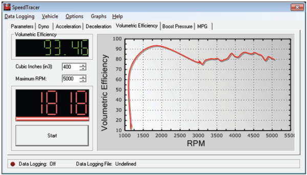
The tool used in this article requires engine size to be entered as cubic inches. Simply multiplying the engine size by 61 provides an answer in liters. Environmental information, such as barometric pressure and ambient temperature should be entered.

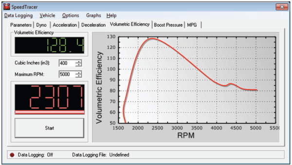
The tool is able to calculate air density, volumetric flow rate, theoretical airflow and VE, as well as keep track of the highest VE and associated rpm.

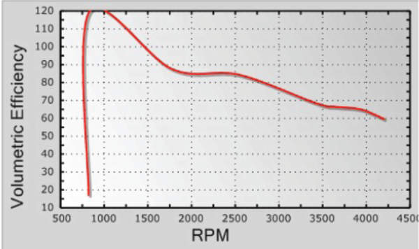
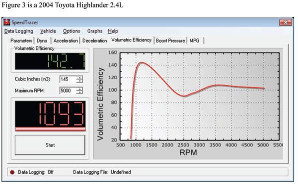
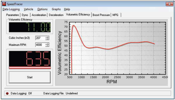
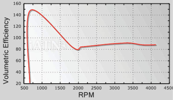
Fig. 1 shows a 2011 Ford Edge 3.5L and is a perfect example of a normal vehicle while set up in a proper starting position. The red tracer is the VE graphing generated by the tool, and I added the MAF sensor information and time from this event’s recording. The orange tracer represents the MAF reading, and the blue line is the time line.

The acceleration event in Fig. 1 lasted about 4.5 seconds.

Notice from idle to about 2,200 rpms that the airflow increases at a sharper rate. We have hit the MAF sensor with a sledgehammer of air. The software recognized the rate at which the air rushed in and depicted the throttle opening event as a sharp rise in VE. The peak reading is 123%.

The VE reacted in such an exaggerated way because the initial rush of air that filled the intake was much larger than what the engine should be flowing at idle rpms.

We know that air must pass the MAF before the engine can make use of it, so add that to any minor data refresh delays and we end up with an obvious spike in VE that depicts the event.

Due to the vehicle setup conditions, throttle snap-open becomes the highest VE capture. This is where we can derive the MAF sensor’s state of health. The rest of the graph depicts how the engine mechanical is able to catch up to the high VE average at the beginning of the event rather than at the end.

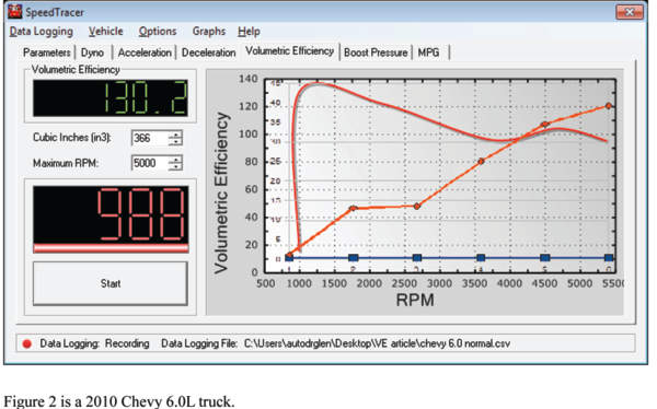
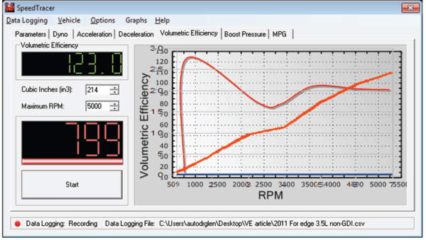
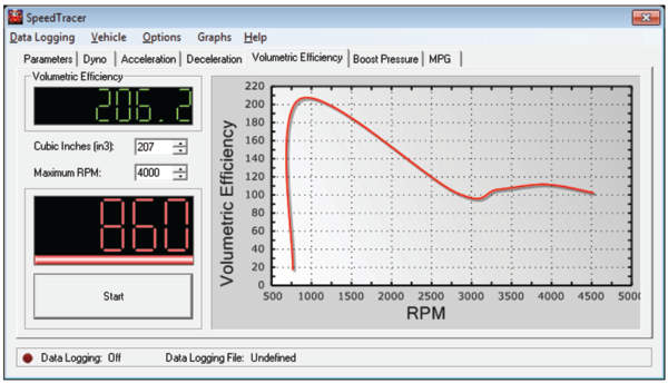
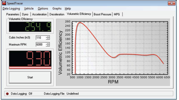
Fig. 2 is a 2010 Chevy 6.0L truck. Fig. 3 is a 2004 Toyota Highlander 2.4L. By now, you should be able to look at these without the MAF tracer added, and we can still identify the events.

Underreporting

Notice how, even though these are completely different vehicles, we can repeat the pattern and put a number range on the MAF.

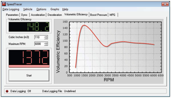
The average length of time of these samples is roughly 4.5 seconds. Within that time, we can detect an underreporting MAF, like the 1999 Toyota 4Runner 3.4L in Fig. 4.

See the difference of a new MAF sensor on the same 3.4L 4Runner in Fig. 5.

Overreporting

We can see an overreporting MAF due to an incorrect replacement MAF sensor on a Toyota Matrix in Fig. 6.

You can see in Fig. 7 that the correct MAF fixed the Matrix.

Restrictions

You can see the partial exhaust restriction in the 2.4L Toyota Highlander’s capture in Fig. 8. This is the same vehicle as Fig. 3, but Fig. 3 (page 38) is post-repair.

You can see in Fig. 8 that we have a good MAF sensor, but something choked the airflow down. Remember the pen and paper method for VE? Would this restricted exhaust have been seen using that method?

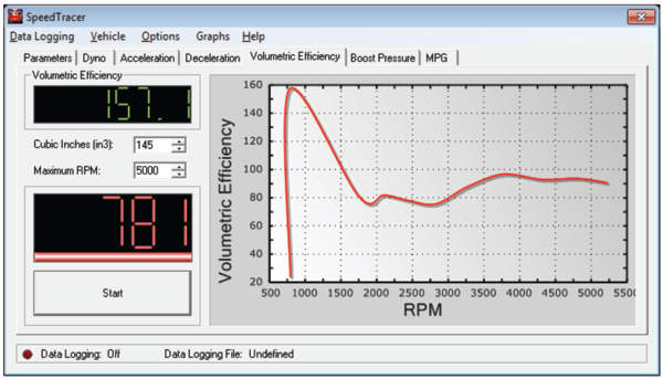
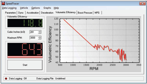
Fig. 9 shows an incorrect Ford Intake Manifold Runner Control (IMRC) linkage setup.

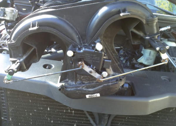
The rods linking the IMRC shafts to the actuator have been reversed on this Ford F-150, so that they are physically closed when commanded open, and vise-versa. When it came time for the IMRC shafts to command open (at 2,500 rpms), they closed off in reality (Fig. 10).

The only clue for this condition using conventional data was that the “feel” of the engine torque lowered when the IMRC changed state. But it is obvious here that something is wrong. We can see the difference in the post-repair capture (Fig. 12). See the correct IMRC rod orientation in Fig. 11.

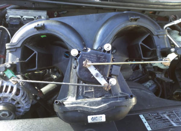
In Fig 13, we have a 4.2L with one CAT completely stopped up.

It would barely register over 3,000 rpms. There was absolutely no practical need for this, but I was curious.

Knowing that only three of the six cylinders can exhale, and that a huge part of the data comes from the MAF readings, what kind of image does that turbulence paint in your mind?

Fig. 14 shows a test subject that suffered catastrophic failure of both CATs. A series of samples were taken while chunks of material were blowing out of the tail pipe. This image repeated multiple times.

Until it ran out of “bullets” (Fig. 15).